



I’m very happy to announce that themis 1.1.0 is now on CRAN. themis provides extra recipes steps for dealing with unbalanced data. You can install it with:
install.packages("themis")This release provides a substantial amount of new features. We will cover the highlights in this blog post, which include: 11 new steps, setting sampling targets per class, and more distance metrics. See the news file for a complete list of changes in this release.
To get started, load the tidymodels and themis packages:
library(tidymodels)
library(themis)

set.seed(1234)
New sampling steps#
This release adds support for 11 new steps for under- and over-sampling of data.
Making for a more complete picture of the commonly discussed methods in this category.
Each step also ships a direct-implementation counterpart (enn(), smogn(), and so on) for use outside a recipe.
The new steps fall into four groups.
Cleaning-based under-sampling removes observations that sit in the wrong neighborhood:
step_enn()applies the Edited Nearest Neighbors rule.step_ncl()applies the Neighborhood Cleaning Rule.step_cnn()uses Condensed Nearest Neighbors.step_oss()uses One-Sided Selection.
Selection-based under-sampling picks a smaller set of representatives instead:
step_cluster_centroids()replaces each class with one representative per k-means cluster.step_instance_hardness()removes the observations that are hardest to classify.
Over-sampling gains three new variants:
step_kmeans_smote()generates new examples only inside clusters where the minority class dominates.step_svmsmote()concentrates them near the decision boundary found by a support vector machine.step_smoten()handles data where every predictor is categorical.
Lastly we have a step that applies the SMOTE idea to regression:
The new “Methods overview” article lays out the full taxonomy.
Sampling targets per class#
The over_ratio and under_ratio arguments used by many of the steps in themis previously only took a single value.
We now accept a named vector,
such that you can specify the value for each level of the outcome.
The penguins data set has three species of unequal size.
A few penguins have missing measurements,
which we drop up front so the counts below are easier to follow:
data(penguins, package = "modeldata")

penguins <- penguins |>
  drop_na()

count(penguins, species)
# A tibble: 3 × 2
species n
<fct> <int>
1 Adelie 146
2 Chinstrap 68
3 Gentoo 119
The names of the vector should correspond to the levels of the outcome.
So over_ratio = c(Chinstrap = 0.8, Gentoo = 1) brings Gentoo up to the size of the majority level,
and Chinstrap up to 80% of it:
recipe(species ~ bill_length_mm + bill_depth_mm + flipper_length_mm + body_mass_g,
       data = penguins) |>
  step_smote(species, over_ratio = c(Chinstrap = 0.8, Gentoo = 1)) |>
  prep() |>
  bake(new_data = NULL) |>
  count(species)
# A tibble: 3 × 2
species n
<fct> <int>
1 Adelie 146
2 Chinstrap 117
3 Gentoo 146
Levels you don’t name are left untouched,
as are rows with a missing outcome.
Two things to keep in mind:
supplying a vector means the argument can no longer be tuned,
and step_rose() still requires a single number,
because its over_ratio scales the size of the total generated sample rather than setting a per-class target.
The new article on over_ratio and under_ratio walks through both arguments in more detail.
Tracking synthetic rows#
Every up-sampling step gains an indicator_column argument.
Give it a name and the final data gets a logical column marking which rows the step added:
smote_res <- recipe(class ~ x + y, data = circle_example) |>
  step_smote(class, indicator_column = "synthetic") |>
  prep() |>
  bake(new_data = NULL)

count(smote_res, class, synthetic)
# A tibble: 3 × 3
class synthetic n
<fct> <lgl> <int>
1 Circle FALSE 58
2 Circle TRUE 284
3 Rest FALSE 342
This will mostly be useful as a diagnostic tool, or to help visualize how these methods work in practice.
smote_res |>
  ggplot(aes(x, y, color = synthetic)) +
  geom_point(alpha = 0.7) +
  labs(
    title = "Synthetic minority observations created by step_smote()",
    color = "Synthetic"
  ) +
  theme_minimal()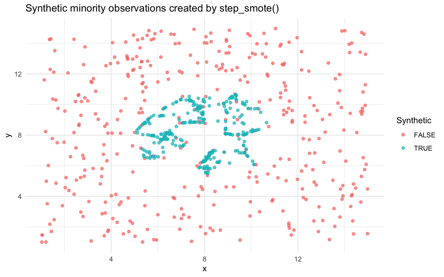
More distance metrics#
Most of the steps in this package are built on some calculation that has to do with nearest neighbors.
And so far all of them had been using Euclidean distances.
We have added a distance argument to every step that deals with neighbors, letting you choose a different distance metric.
manhattan_res <- recipe(class ~ x + y, data = circle_example) |>
  step_smote(class, distance = "manhattan", indicator_column = "synthetic") |>
  prep() |>
  bake(new_data = NULL)

count(manhattan_res, class, synthetic)
# A tibble: 3 × 3
class synthetic n
<fct> <lgl> <int>
1 Circle FALSE 58
2 Circle TRUE 284
3 Rest FALSE 342
The class counts are unchanged,
since those are set by over_ratio rather than by the metric.
What changes is where the synthetic observations land,
because a different metric picks different nearest neighbors to interpolate between.
Acknowledgements#
A big thank you to everyone who has contributed issues, pull requests, and discussion since the last release! @3styleJam, @Dodothereal, @EmilHvitfeldt, @FvD, @jeroenjanssens, @SAY-5, and @topepo.