Measure model performance with yardstick

Intro#

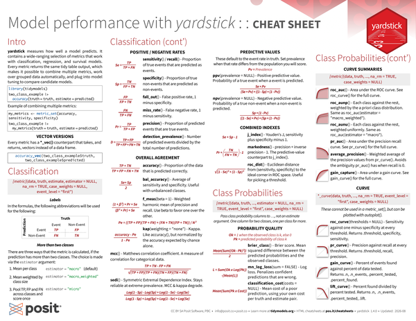
yardstick measures how well a model predicts. It contains a wide-ranging selection of metrics that work with classification, regression, and survival models.

Every metric returns the same tidy table output, which makes it possible to combine multiple metrics, work over grouped data automatically, and plug into model tuning to compare candidate models.

library(tidymodels)

two_class_example |>
  accuracy(truth = truth, estimate = predicted)

Example of combining multiple metrics:

my_metrics <- metric_set(accuracy, sensitivity, specificity)

two_class_example |>
  my_metrics(truth = truth, estimate = predicted)

Vector versions#

Every metric has a *_vec() counterpart that takes, and returns, vectors instead of a data frame.

accuracy_vec(two_class_example$truth, two_class_example$predicted)

Classification#

[metric](data, truth, estimate, estimator = NULL, na_rm = TRUE,
         case_weights = NULL, event_level = "first")

Labels#

In the formulas, the following abbreviations will be used for the following:

	Prediction: Event	Prediction: Non-Event
Truth: Event	`TP`	`FN`
Truth: Non-Event	`FP`	`TN`

More than two classes#

There are three ways that the metric is calculated, if the prediction has more than two classes. The choice is made via the estimator argument:


Mean per class (default)	`estimator = "macro"`
Mean weighted by class size	`estimator = "macro_weighted"`
Pool TP, FP and FN across classes and score once	`estimator = "micro"`

Overall agreement#

accuracy(): Proportion of the data that is predicted correctly.
```
(TP + TN) / (TP + FP + FN + TN)
```
bal_accuracy(): Average of sensitivity and specificity. Useful with unbalanced classes.
```
(Se + Sp) / 2
```
f_meas(beta = 1): Weighted harmonic mean of precision and recall. Use beta to favor one over the other.
```
((1 + β²) × Pr × Se) / ((β² × Pr) + Se)
```
kap(weighting = "none"): Kappa. Like accuracy(), but normalized by the accuracy expected by chance alone.
```
(accuracy - Pe) / (1 - Pe)
```
Where Pe = ((TP + FP)(TP + FN) + (FN + TN)(FP + TN)) / N².
mcc(): Matthews correlation coefficient. A measure of correlation for categorical data.
```
(TP × TN - FP × FN) / √((TP + FP)(TP + FN)(TN + FP)(TN + FN))
```
sedi(): Symmetric Extremal Dependence Index. Stays reliable at extreme prevalence, where MCC and kappa degrade.
```
(Log(1 - Sp) - Log(Sp) + Log(1 - Se) - Log(Se)) / (Log(1 - Sp) + Log(Sp) + Log(1 - Se) + Log(Se))
```

Positive / negative rates#

sensitivity() / recall(): Proportion of true events that are predicted as events.
```
Se = TP / (TP + FN)
```
specificity(): Proportion of true non-events that are predicted as non-events.
```
Sp = TN / (FP + TN)
```
fall_out(): False positive rate, 1 minus specificity.
```
FP / (FP + TN)
```
miss_rate(): False negative rate, 1 minus sensitivity.
```
FN / (TP + FN)
```

Predictive values#

These default to the event rate in truth. Set prevalence when that rate differs from the population you will score. In the formulas, Pv is the prevalence.

ppv(prevalence = NULL): Positive predictive value. Probability of a true event when an event is predicted.
```
(Se × Pv) / ((Se × Pv) + ((1 - Sp) × (1 - Pv)))
```
npv(prevalence = NULL): Negative predictive value. Probability of a true non-event when a non-event is predicted.
```
(Sp × (1 - Pv)) / (((1 - Se) × Pv) + (Sp × (1 - Pv)))
```
precision(): Proportion of predicted events that are true events.
```
Pr = TP / (TP + FP)
```
detection_prevalence(): Number of predicted events divided by the total number of predictions.
```
D = (TP + FP) / (TP + FP + FN + TN)
```

Combined indexes#

j_index(): Youden’s J, sensitivity plus specificity minus 1.
```
Se + Sp - 1
```
markedness(): Precision plus inverse precision, minus 1. The predictive-value counterpart to j_index().
```
(Pr + (TN / (FN + TN))) - 1
```
roc_dist(): Euclidean distance from (sensitivity, specificity) to the ideal corner in ROC space. Useful for picking a threshold.
```
√((1 - Se)² + (1 - Sp)²)
```

Class Probabilities#

[metric](data, truth, ..., estimator = NULL, na_rm = TRUE,
         event_level = "first", case_weights = NULL)

Pass class probability columns to ..., not an estimate argument. One column for two classes, one per class for more.

Probability quality#

In the formulas, Ok is 1 when the observed class is k and 0 otherwise, and Pk is the predicted probability of class k.

brier_class(): Brier score. Mean squared difference between the predicted probabilities and the observed classes.
```
Mean(Sum((Ok - Pk)²)) / 2
```
mn_log_loss(sum = FALSE): Log loss. Penalizes confident predictions that are wrong.
```
-(Mean(L))
```
Where L = Sum(Ok × Log(Pk)).
classification_cost(costs = NULL): Mean cost of a poor prediction, using your own cost per truth and estimate pair.
```
Mean(Sum(Pk × Cost))
```

Curve summaries#

[metric](data, truth, ..., na_rm = TRUE, case_weights = NULL)

roc_auc(): Area under the ROC curve. See roc_curve() for the full curve.
roc_aunp(): Each class against the rest, weighted by the a priori class distribution. Same as roc_auc(estimator = "macro_weighted").
roc_aunu(): Each class against the rest, weighted uniformly. Same as roc_auc(estimator = "macro").
pr_auc(): Area under the precision recall curve. See pr_curve() for the full curve.
average_precision(): Weighted average of the precision values from pr_curve(). Avoids the ambiguity pr_auc() has when recall is 0.
gain_capture(): Area under a gain curve. See gain_curve() for the full curve.

Curves#

*_curve(data, truth, ..., na_rm = TRUE, event_level = "first",
        case_weights = NULL)

These cannot be used in a metric_set(), but can be plotted with autoplot().

roc_curve(thresholds = NULL): Sensitivity against one minus specificity at every threshold. Returns .threshold, specificity, sensitivity.
pr_curve(): Precision against recall at every threshold. Returns .threshold, recall, precision.
gain_curve(): Percent of events found against percent of data tested. Returns .n, .n_events, .percent_tested, .percent_found.
lift_curve(): Percent found divided by percent tested. Returns .n, .n_events, .percent_tested, .lift.

Regression#

[metric](data, truth, estimate, na_rm = TRUE, case_weights = NULL)

In the formulas, Tr is the truth, Es is the estimate, and Er is the error (Tr - Es).

Error#

mae(): Mean absolute error.
```
Mean(Abs(Er))
```
msd(): Mean signed deviation. Averages the signed differences, it measures bias not size of error.
```
Mean(Er)
```
mse(): Mean squared error.
```
Mean(Er²)
```
rmse(): Root mean squared error.
```
Rm = √Mean(Er²)
```
rmse_relative(): RMSE normalized by the range of the true values. Also called NRMSE.
```
Rm / (Max(Tr) - Min(Tr))
```
mase(m = 1L, mae_train = NULL): Mean absolute scaled error. Scale independent, for forecast error. Order rows by time first.
```
Mean(Abs(Er)) / Mean(Abs(Tr - Lag(Tr, m)))
```
mpe(): Mean percent error. Signed, so it measures bias. Returns Inf if any truth value is 0.
```
Mean2(Er / Tr)
```
Where Mean2(x) = Mean(x) × 100.
mape(): Mean absolute percent error.
```
Mean2(Abs(Er / Tr))
```
smape(): Symmetric mean absolute percent error.
```
Mean2((2 × Abs(Er)) / (Abs(Tr) + Abs(Es)))
```

Agreement and correlation#

rsq(): R squared, computed from the correlation. Between 0 and 1.
```
Cor(Tr, Es)²
```
rsq_trad(): R squared, computed from sums of squares. Can go negative.
```
Sum((Tr - Es)²) / Sum((Tr - Mean(Tr))²)
```
ccc(bias = FALSE): Concordance correlation coefficient. Measures agreement with the 45 degree line, not just correlation.
```
(2 × Cov(Tr, Es)) / (Var(Tr) + Var(Es) + (Mean(Tr) - Mean(Es))²)
```
rpd(): Ratio of performance to deviation. Consistency with the observed values, not accuracy.
```
Sd(Tr) / Rm
```
rpiq(): Ratio of performance to inter-quartile.
```
IQR(Tr) / Rm
```
iic(): Index of ideality of correlation. Combines the correlation with the mean absolute error.
```
Cor(Tr, Es) × (Min(Mn, Mp) / Max(Mn, Mp))
```
Where Mp = Mean(Abs(Positive Er)) and Mn = Mean(Abs(Negative Er)).

Robust to outliers#

huber_loss(delta = 1): Quadratic for small residuals, linear for large ones. Less sensitive to outliers than rmse().
huber_loss_pseudo(delta = 1): Smooth approximation of huber_loss().

Ranking and counts#

gini_coef(): Normalized Gini coefficient. Measures ranking ability from the Lorenz curve. Used for risk and loss cost models.
poisson_log_loss(): Log loss for count outcomes, using the Poisson distribution.

Fairness#

[metric](by)

Each builds a metric, not a value. Pass the protected group column unquoted to by, then use it like any metric. 0 means equal scores across groups. In the formulas, g is the protected group and Range(x) is Max(x) - Min(x).

demographic_parity(): Range of detection_prevalence() across groups. Same predicted positive rate everywhere. Ignores the true outcome.
```
Range(D(g))
```
equal_opportunity(): Range of sensitivity() across groups. Same true positive rate everywhere.
```
Range(Se(g))
```
equalized_odds(): Largest range of sensitivity() or specificity() across groups. Same error rates of every kind.
```
Max(Range(Se(g)), Range(Sp(g)))
```
new_groupwise_metric(fn, name, aggregate, direction = "minimize"): Build your own from any metric function, summarizing its per group values with aggregate.

Survival#

All of these are for right censored data. Pass a survival::Surv() object to truth.

Dynamic predictions#

[metric](data, truth, ..., na_rm = TRUE, case_weights = NULL)

Pass the list column of predicted survival probabilities from a censored model to .... Results come back one row per .eval_time.

brier_survival(): Mean squared error at each evaluation time.
brier_survival_integrated(): One Brier score across all evaluation times.
roc_auc_survival(): Area under the ROC survival curve at each evaluation time.
roc_curve_survival(): The full ROC survival curve, for plotting.

Static and linear predictor#

[metric](data, truth, estimate)

concordance_survival(): Concordance index. Ranking ability across the whole follow-up, with no evaluation time.
royston_survival(): Royston-Sauerbrei D statistic. Separation between risk groups, from a linear predictor.

Other metrics#

Ordinal#

ranked_prob_score(data, truth, ..., na_rm = TRUE, case_weights = NULL): Ranked probability score. truth is an ordered factor; ... takes one probability column per level, in order. Credits near misses.

Quantile#

weighted_interval_score(data, truth, estimate, quantile_levels = NULL, na_rm = TRUE, quantile_estimate_nas = "impute", case_weights = NULL): Quantile based approximation of the continuous ranked probability score. Generalizes absolute error.

Operations#

library(tidymodels)

Metric sets#

metric_set(...): Combines metric functions into one function that computes all of them at once. Only compatible types can be mixed.
```
class_mets <- metric_set(accuracy, sensitivity, specificity)
```
get_metrics(type): Returns a metric_set() of every metric of the given type, such as "class" or "prob".
```
class_mets <- get_metrics("class")
```
metrics(data, truth, estimate, ...): Computes a default set of metrics, chosen by the class of truth.
```
metrics(hpc_cv, obs, pred)
```
metric_tweak(.name, .fn, ...): Presets optional arguments on a metric. Do this before the metric goes into a metric_set(), since you cannot change them afterwards.
```
f2 <- metric_tweak("f2", f_meas, beta = 2)
```

Confusion matrix#

conf_mat(data, truth, estimate, dnn = c("Prediction", "Truth")): Cross tabulates observed against predicted classes.
```
cm <- conf_mat(hpc_cv, obs, pred)
```
summary(object, prevalence = NULL, beta = 1, estimator = NULL, event_level = "first"): Computes most of the classification metrics at once from the matrix.
```
summary(cm)
```
tidy(x): Turns the matrix into a tibble with one row per cell.
```
tidy(cm)
```
autoplot(object, type = "mosaic"): Draws the matrix. Use type = "heatmap" for the other style.
```
autoplot(cm, type = "heatmap")
```