New tidymodels Releases for April 2026

We’ve released a sequence of tidymodels packages over the last few weeks: dials (1.4.3), parsnip (1.5.0), tune (2.1.0), yardstick (1.4.0), and tidymodels (1.5.0). You can install them via:

1
2
3


# tidymodels installs all of the new versions
require(pak)
pak::pak("tidymodels")

Here are links to the NEWS files for each package:

Let’s first talk about the two biggest updates enabled by this group of releases, then we’ll cover some of the other changes for each package.

Ordered Outcomes#

parsnip has a new model type, ordinal_reg(), analogous to multinom_reg(), for fitting various generalized linear models with ordered class levels.

The ordered package by Cory Brunson is now on CRAN. This contains the specific engine code for these models, including:

ordinal_reg(): three engines: "polr", "ordinalNet", and "vglm".
gen_additive_mod(): "vgam"
decision_tree(): "rpartScore"
rand_forest(): "ordinalForest"

These models can be fitted, tuned, and evaluated with tidymodels. For the evaluation, we’ve added a specific performance metric for ordered categories: the ranked probability score (RPS). The function ranked_prob_score() is in the new yardstick release and requires an ordered factor for the outcome.

Quantile Regression#

We previously reported that parsnip supports quantile regression models. With the latest set of releases, new boosting and neural network engines are available, and these models can now be tuned and evaluated using a relevant metric. yardstick now includes the weighted interval score ( Bracher et al (2021) ) to evaluate the quality of the quantile predictions.

Here’s a simple one-dimensional example using the Ames data; we’ll predict the sale price as a function of latitude. To start, let’s make a training/test split, generate some resamples, and plot the training data.

 1
 2
 3
 4
 5
 6
 7
 8
 9
10
11
12
13
14
15
16
17


library(tidymodels)
# We'll also need the qrnn package for the neural network engine

set.seed(1215)
ames_split <-
  ames |>
  select(Latitude, Sale_Price) |>
  initial_split(strata = Sale_Price)
ames_train <- training(ames_split)
ames_test <- testing(ames_split)
ames_rs <- vfold_cv(ames_train, strata = Sale_Price)

ames_train |>
  ggplot(aes(Latitude, Sale_Price)) +
  geom_point(alpha = 1 / 5) +
  geom_smooth(se = FALSE) +
  labs(x = "Latitude", y = "Sale Price (USD)")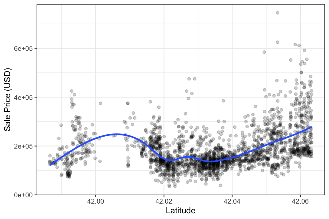

Note that we almost always model these data with a log transformation on the outcome due to its inherent skewness. That helps us avoid making negative predictions, be more robust to overly influential points (i.e., locations with very large sale prices), and stabilize the variance. However, we don’t necessarily have to do that with quantile regression. The objective functions used to estimate parameters do not impose requirements on the normality of the data or heterogeneity of residuals. For this analysis, let’s stick with the original units of the outcome (USD).

There are a few engines for quantile regression, and we’ll use a neural network model. To get started, the quantiles to be predicted need to be specified. We make a model specification with a few additions:

 1
 2
 3
 4
 5
 6
 7
 8
 9
10
11
12
13
14
15
16
17
18


# Pre-defined quantiles of interest
qnt_lvls <- c(0.05, 0.25, 0.5, 0.75, 0.95)

nnet_spec <-
  mlp(hidden_units = tune(), penalty = tune(), epochs = 10) |>
  # Set the quantile levels with the mode:
  set_mode("quantile regression", quantile_levels = qnt_lvls) |>
  # A new engine for quantile regression with neural networks via the
  # qrnn package. We'll add an engine argument to specify the
  # optimization method for training the model:
  set_engine("qrnn", method = "adam")

# Scale the single predictor to help the model initialize its
# parameters.
nnet_rec <- recipe(Sale_Price ~ ., data = ames_train) |>
  step_normalize(all_predictors())

nnet_wflow <- workflow(nnet_rec, nnet_spec)

From there, we can use any of our tuning functions to optimize the number of hidden units and the amount of weight decay. By default, the weighted interval score is used for this particular mode.

We’ll consider 25 tuning parameter candidates to optimize model performance.

1
2
3
4
5
6
7
8


set.seed(971)
nnet_res <-
  nnet_wflow |>
  tune_grid(
    resamples = ames_rs,
    grid = 25,
    control = control_grid(save_workflow = TRUE)
  )

We can get the performance metric and visualize which tuning parameter combinations have the smallest weighted interval score:

1
2
3
4
5
6
7
8


nnet_mtr <- collect_metrics(nnet_res)

nnet_mtr |>
  ggplot(aes(penalty, hidden_units, size = mean)) +
  geom_point() +
  scale_x_log10() +
  coord_fixed(ratio = 1) +
  labs(x = "Penalty", y = "# Hidden Units", size = "WIS")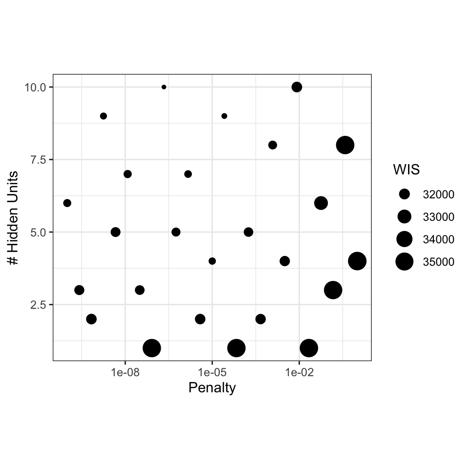

1

select_best(nnet_res, metric = "weighted_interval_score")

# A tibble: 1 × 3
  hidden_units     penalty .config         
         <int>       <dbl> <chr>           
1           10 0.000000215 pre0_mod24_post0

The model appears to prefer a smaller penalty and more hidden units.

It’s hard to conceptualize how well the model functions with just these numbers. To show that the metric does select good models, let’s fit the best, median, and worst models and see how they look on the test set.

 1
 2
 3
 4
 5
 6
 7
 8
 9
10
11
12
13
14
15
16
17
18
19


set.seed(8281)
best_model <- fit_best(nnet_res)

set.seed(8281)
worst_model <-
  nnet_mtr |>
  slice_max(mean, n = 1) |>
  select(hidden_units, penalty) |>
  finalize_workflow(nnet_wflow, parameters = _) |>
  fit(ames_train)

set.seed(8281)
mid_model <-
  nnet_mtr |>
  # Since we have an odd number of grid points:
  filter(mean == median(mean)) |>
  select(hidden_units, penalty) |>
  finalize_workflow(nnet_wflow, parameters = _) |>
  fit(ames_train)

Now let’s plot the results. We’ll color the predicted quantiles: black indicates the predicted median sale price, orange lines indicate the inner quartiles, and smoky periwinkle lines indicate the 0.05 and 0.95 quantiles (which could serve as 90% prediction intervals).

 1
 2
 3
 4
 5
 6
 7
 8
 9
10
11
12
13
14
15
16
17
18
19
20
21
22
23
24
25


bind_rows(
  best_model |> augment(ames_test) |> mutate(Model = "Best Results"),
  mid_model |> augment(ames_test) |> mutate(Model = "Meh Results"),
  worst_model |> augment(ames_test) |> mutate(Model = "Worst Results")
) |>
  mutate(
    .pred_quantile = map(.pred_quantile, ~ as_tibble(.x))
  ) |>
  unnest(.pred_quantile) |>
  arrange(Latitude) |>
  ggplot(aes(Latitude)) +
  geom_point(aes(y = Sale_Price), alpha = 1 / 30, cex = 3 / 4) +
  geom_path(
    aes(
      y = .pred_quantile,
      group = .quantile_levels,
      col = factor(.quantile_levels)
    ),
    show.legend = FALSE,
    linewidth = 1
  ) +
  scale_color_manual(
    values = c("#8785B2FF", "#D95F30FF", "black", "#D95F30FF", "#8785B2FF")
  ) +
  facet_wrap(~Model)

These plots show that configurations with very large score values have poor fits (linear in this case). The “meh” model is nonlinear but not responsive enough to the datas’ ups and downs. The best model, with more hidden units and a low penalty, appears to be flexible enough to model the data well.

We’ll have more metrics in yardstick that can use quantile predictions in the future. For example, we can extend the ones that we have, such as rmse() or rsq(), to use a predicted value from the center of the predictive distribution, such as the 0.5 quantile.

Now we’ll describe various other improvements in the recently released versions.

dials#

The latest dials release contains several new parameters for new-ish models in parsnip: For the ordinal_reg() models, dials now contains ordinal_link() and odds_link(). For the tab_pfn(), dials contains num_estimators(), softmax_temperature(), balance_probabilities(), average_before_softmax(), and training_set_limit().

The other user-facing changes were related to input checking and related error messages. The most prominent example is that parameters() and the grid_*() functions now give more information in the error message when non-parameter objects are passed in: which inputs aren’t a parameter object and what they are instead.

@corybrunson , @daltonkw , @hfrick , @jeroenjanssens , @topepo , and @vmikk contributed to the package since the last release.

yardstick#

Beyond the two new metrics ranked_prob_score() and weighted_interval_score() described above, this release adds a further 8 metrics.

Three new regression metrics:

mse() — mean squared error (the squared counterpart to the existing rmse()).
rmse_relative() — root mean squared error normalized by the observed value range.
gini_coef() — normalized Gini coefficient.

Three new classification metrics:

fall_out() — false positive rate (1 − specificity).
miss_rate() — false negative rate (1 − sensitivity).
markedness() — predictive power of a classifier, computed as PPV + NPV − 1.

Two new probability-based classification metrics:

roc_dist() — Euclidean distance from the perfect-classifier corner of ROC space.
sedi() — Symmetric Extremal Dependence Index.

In addition to these new metrics, we have also updated the documention of all metrics. Now each metric shows the formula used to calculate it, as well as the valid values it can produce.

We also have pages that list all metrics of the same type. These can be found with ?class-metrics , ?numeric-metrics or linked within each metric documentation.

We are thankful to the developers who contributed to this version: @abichat , @astamm , @corybrunson , @DarioS , @EmilHvitfeldt , @FvD , @hfrick , @JavOrraca , @jeroenjanssens , @jkylearmstrong-temple , @mle2718 , @nathant181 , @SimonDedman , @topepo , and @tripartio

parsnip#

Version 1.5.0 of parsnip had a variety of changes. Besides the additions for the two new model types shown above:

We enabled case weight usage for the "nnet" engines of mlp() and bag_mlp() as well as for the "dbarts" engine of bart().

Many of the other changes are most likely to be noticed by developers:

The interface for declaring tunable parameters has been simplified and is the same for main arguments as well as engine parameters. Also, these values can now be set inside extension packages.
We now export the generics for predict_quantile(), predict_class(), predict_classprob(), and predict_hazard().
format_predictions() is a new unified function for formatting prediction outputs, consolidating the logic from the individual format_*() functions. The individual functions format_num(), format_class(), format_classprobs(), format_time(), format_survival(), format_linear_pred(), and format_hazard() are now deprecated.

Thanks to those who contributed to parsnip since the last release: @CeresBarros , @corybrunson , @EmilHvitfeldt , @hfrick , @iamYannC , @jack-davison , @jameslamb , @martinju , and @topepo .

tune#

The core functionality of tune is to do all the model fitting (including pre- and postprocessing) and performance evaluation across various resamples and tuning parameter combinations. For grid search, we could take the full parameter grid, splice one parameter combination into the workflow at a time, and run with it. That can be pretty inefficient though. So what actually happens in tune are a few optimizations in how we do all that fitting and evaluating: For preprocessing, we do it once for a resample (per preprocessing parameter combination) and then evaluate all model candidates on it. This lets us avoid unnecessarily repeating the same preprocessing multiple times. For model fitting, we make use of what Max calls “the submodel trick” : For certain models, like a boosted tree, you can use a submodel to make predictions without having to refit the model. A boosted tree ensemble fitted with 20 trees can be used to make predictions for any number of trees up to the 20 used for fitting. That allows us to evaluate different tuning parameter candidates for, here, the number of trees, without having to refit the model. When we added postprocessing, we temporarily disabled this (to ensure we got the integration right) - now we’ve brought it back. We make use of this speedup for both the main model as well as the calibration model.

Another big update is that the Gaussian process model package was changed from GPfit to GauPro because the former is no longer actively maintained. There are some differences:

Fit diagnostics are computed and reported. If the fit quality is poor, an “uncertainty sample” that is furthest away from the existing data is used as the new candidate.
The GP no longer uses binary indicators for qualitative predictors. Instead, a “categorical kernel” is used for those parameter columns. Fewer starting values are required with this change.
For numeric predictors, the Matern 3/2 kernel is always used.

Some other changes of note:

When calculating resampling estimates, we can now use a weighted mean based on the number of rows in the assessment set thanks to Tyler Burch. You can opt-in to this using the new add_resample_weights() function. See ?calculate_resample_weights
The warning threshold when check the size of a workflow is now a parameter to the control functions and has a new default of 100MB.

Some bug fixes:

Models with submodel parameters would train all calibration models on predictions from a single submodel value instead of the correct value for each submodel. We sorted this out.
We fixed a bug for cases where we tune a grid without a model parameter but with a postprocessing parameter.
Another bug was fixed for augment() when using last_fit() objects

Thanks to the following contributors: @edgararuiz , @EmilHvitfeldt , @hfrick , @jeroenjanssens , @jjcurtin , @mikewolfe , @mthulin , @ncalliencsu , @rvalieris , @StevenWallaert , @tjburch , and @topepo